This compression aims at reducing the file sizes as much as possible while preserving the details responsible for image subject's recognisability.

This is an experiment I have done. And there could be better algorithms of this kind.

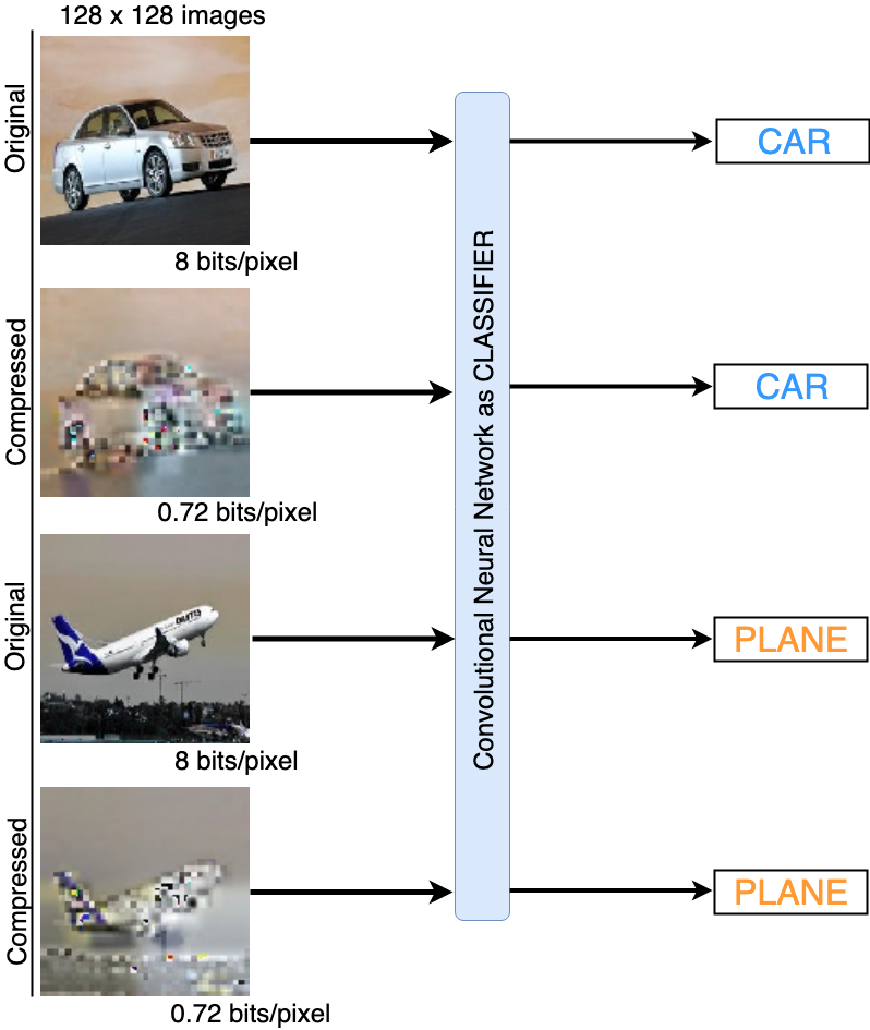
Looking at both the compressed images, you can still recognise a car in the first one and a plane in the second one but they only hold minimal information of about 0.72 bits/pixel instead of their original counterparts occupying 8 bits/pixel.

Obviously you dont want your vacation photos to be compressed this way. This can be more useful in image searching. For example, in Google photos, when we type "car" in the search bar it returns all of our personal photos with a car in it. So, when we search for a car, it just runs through its pre-labelled photos and finds all the photos with "car" tag on it. Lets say Google wanted to add a new label "pet" 🐶 to let every one search their pets pictures. They will probably search all large images in every google account and apply "pet" tag to the images with pets .

This is when the above type of compression comes handy. If we search on smaller readily available image files with recognisable subjects, tagging can be much faster. So we need a compression algorithm which preserves image subject identifiability while having less compute intensive decompression technique.

We will go through the designing of such algorithm, but before trying to understand it, there are few things we need to have a clear picture of.

Things to know:

There are tons of image compression algorithms in use, like DCT, JPEG, HEIF and etcetera which can perform lossy image compressions by ignoring the high frequency components of image. By definition, High-frequency (HF) components correspond to "fine" details in the image while low-frequency(LF) components corresponds to "coarse" details. HF components occupy more disk space (memory) than LF components does. A simple image decomposition into coarse and fine details can be done as shown.

Above equation of images delineates the basic difference between HF & LF in images. Furthermore, the details of images can be separated into images corresponding to multiple frequency bands.

DCT, JPEG & HEIF algorithms discards some of the HF/fine details in an image to reduce the image file size. Desperately compressing images to very small sizes (like less than 1 kb) with these algorithms may result in losing the recognisability of the subject in the image. In simpler words if we compress a 1MB cat photo to 1KB photo, we might not recognise a cat in the final image.

Here I am explaining a lossy image compression model which reduces the image inmemory-size but still preserving the cat details. That means, a human or a computer who reads the compressed image must be able to recognise the subject in it (may be a dog or a cat or a car).

Pyramid Decompositions

Gaussian Pyramids

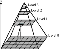
Pooling down an image multiple times using Gaussian filter produces multiple smaller images with exponentially decreasing sizes. All such pooled down images if put one on another forms a pyramid kinda shape.

Laplacian Pyramids

In gaussian pyramids, as we go up the pyramid, finer details (sharp edges or HF noises) are discarded. That means as we go down the pyramid, fined details are added from layer to layer. The concept of Laplacian pyramid is to separate out the finer details which are added to lower levels.

So each N^th Laplacian layer is the difference of upscaled N+1^th and N^th Gaussian layers.

These two are linear multi-scale image decomposition models. There are other pyramids which can capture the edges into a filter based on the orientation of edges. These are called multi-scale, multi-orientation image decomposition models. Example: QMF Wavelet pyramids & Steerable Pyramids. More about pyramids here.

The levels(decoimposed images) of the laplacian pyramid can be compressed since each level in the pyramid has low variance and entropy and each level image may be represented at very low sample density.

Laplacian levels have low variance because, each level mostly stores only the edges, and is filled with near-zero values. Only few number of pixels lying on the edges are away from zero. This means we don’t need 255 values (8 bits) to represent a pixel in each colour channel. Thus we can save some bits by decreasing the color levels. This process is called quantisation.

Convolutional Neural Networks

CNNs are the most famous algorithms among biologically inspired AI techniques. Deep CNN are proved to be very similar to Human visual cortex, which means we can make a computer recognise an image the same way we Humans recognise objects with our eyes. Thus we can instruct the computer to return the recognisability factor of a subject in the image.

In this post, I will be using the CNN for the same purpose: To evaluate the recognisability of a subject(cat or dog / car or plane) during compression process.

Compression Model

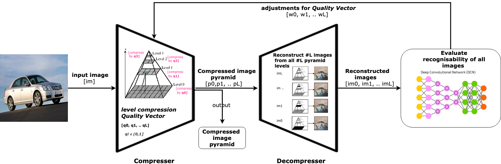
Unlike JPEG compression which is loosely based on human psycho-visual system, we will direct this image compression directly with the CNNs feedback on image recognisability.

First we decompose the image into multiple levels of laplacian pyramids. Now we check the proportions of all layers contributing to image recognisability. The layer which is contributing the least will be compressed (lossily) more. Now again we will check the contributions of each layer to the image’s recognisability and re adjust the proportions. This will be repeated until the CNN shows enough ambiguity in recognition. Finally, we will compress all the pyramid layers(lossily) in the optimal proportions.

Compression Algorithm

To explain in layman terms, we decompose the image into multiple levels of details and evaluate each detail on its usefulness in forming a recognisable image. Next we discard some part of the less useful details from the image.

Step wise:

Decompose the image into multiple details. Here we will take laplacian pyramid levels to decompose image based on frequency bandwidth. Here, I have decomposed a car image upto 5 laplacian levels where each level contains details corresponding to a band of frequencies.
All level 0 details corresponds to high frequency changes in the image, that is, mostly sharp edges. All subsequent levels corresponds to lower frequencies. The very upper layer, (level 5 here) simpy contains mostly the average background color.

Each layer has its own importance in contributing to the scene of the image. As well as they have some unnecessary details. For example, level 0 which picks up high frequencies, is likely to pickup noise which is an unnecessary detail. And, level 5 will pick up the colors of the subject's background which is again a non contributing detail (noise).

Now we want to know how much unnecessary details each layer contains, so that we can drop details in each layer proportionately.
For finding the dose of unnecessary detais in each layer, we do this:

From the laplacian pyramid, drop off some details in the intended layer. We can do this by using a lossy compression where we control the amount of quality drop. JPEG is a good example for this kinda usecase. Not only JPEG, but we can do multiple experiments by using multiple image compression techniques .
Next, we reconstruct the image from the compressed layer and other non-compressed layers
Feed both the original image and reconstructed image to CNN and compare the confidence values returned by it. If the confidence drop is more, that means the compressed pyramid layer contributes more to the image recognisability. If its less, then it is the other way around.
Less is the drop of confidence, more is the amount of unnecessary details in the layer. So we choose to compress it more than other layers.

The compressed pyramid will be the new pyramid again. We repeat the process until there is a significant reduction in confidence values. The final pyramid will be returned for storage. And yes, there is a further scope of compressing each layers losslessly with available fast compression-decompression algorithms.

Outcome

The laplacian pyramid is created for the required input image. In the first iteration each layer of the image pyramid contains 100% of its details. In subsequent iterations, we calculate the weightage of non-contributing details in each level and partially drop off some info using lossy compression on each level.

Here I used naive resizing, quantizing & jpeg compressions to compress the pyramids.

The compression runs untill the CNN's confidence decreases to 60% of its initial. Or may be what ever the treshold we put.
We can carry-out the same compression algorithm with different lossy compression techniques (as explained in step 2) .

With naive cv2's resize as the lossy compression technique:

compressedPyramid[layerNo] = 
cv2.resize(compressedPyramid[layerNo], newShape, interpolation=cv2.INTER_NEAREST)

The final compression ratios of the levels of pyramid ended up this way

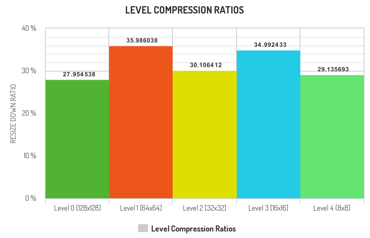
There are couple of interpretations we can draw from this graph:

Level 0 was compressed more than other layers. This could be because, the high frequency details in level 0 is contributing less to the overall recognisability of the image.
A simple example for this is the texture of the subject. You dont need to see the texture of the plane, to say the image conatins a plane.
Without level 0, the image simply gets blurred, but we still see the plane.
Next to the level 0, level 4 was compressed more. Again the interpretation goes like this:
Level 4 is a 8x8 pixel image, it mostly contains the average colors of the image. Loosing some color details in the image should not trick us into classifying the image wrong.
Without level 4, the reconstructed image looses some of the overall color details.

Using pixel value quantisation as the lossy compression technique:

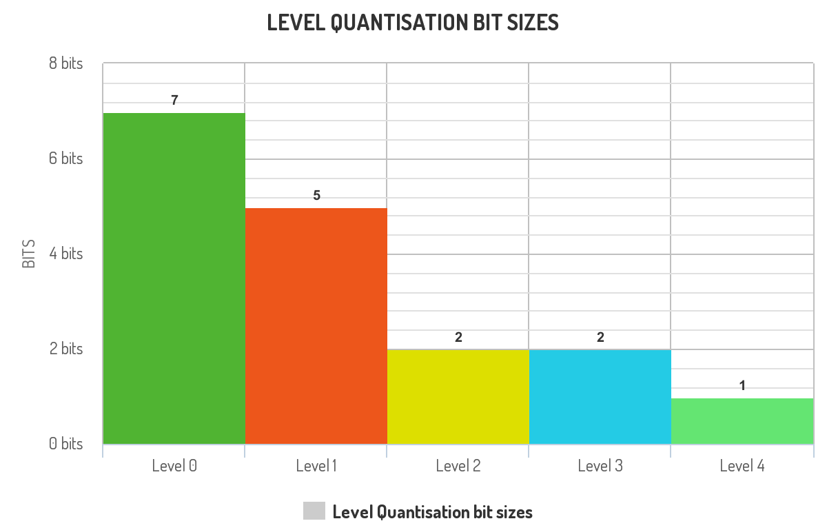
Quantising pixels values will restrict the number of colors visible in the image.

Interpretations from the graph:

Level 0 is the least compressed of all in the pyramid because quantizing the level 0 will introduce high-frequency noise, which confuses the CNN. This happens due to pixel values of all the sharp edges taking the nearest avaliable colors.
This decreasing compression rations in the graph can be explained with entropy. Entropy(H) is 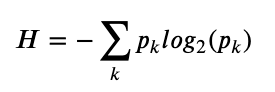where K is the number of gray levels and p_k is the ratio of '#pixels with graylevel k' to '#pixels in image'. → As we go up the laplacian pyramid, the entropy of the image decreases [paper]
→ Quantisation decreases the number of available gray levels, thus decreasing the entropy. So, quantisation is a entropy reducer.
→ Quantising the lower layers of pyramids has more effect on image entropy than on upper layers.
→ So, the above compression algorithm has decreasewd entropy of higher levels more than the entropy of lowerlevels.

results

After compressing a set of 128x128 sized images using combination of the above explained techniques, the pyramids were compressed to 393216 Bits. That is an quaivalent of (0.72 Bits/pixel).

A faster CNN which directly consumes the compressed pyramids can be developed for faster image classifications. This type of CNN consumes the upper layers of pyramid in different stages of its sequential model. This is possible by using hybrid hidden layers which also takes direct input. Thus we can reduce the overall classification time and power needed. (This will be my future work)

The total purpose of this spare-time work is to learn & analyze the decompositions and the role of each decomposed image in recognisability. The compression model discussed here is a very rudimentary one, as it only decomposes the image based on frequencies. We can employ other types of image decomposition techniques to make this work better.

If we really want to throw away unnecessary details, we can completely eliminate the background of the image. This can be achieved by using Image segmentation rather than image decomposition.